after-hours

What I build when I am bored.

Nobody assigned any of it and none of it is coursework: it is what a free evening turns into, in machine learning, computer algebra and applied mathematics. Each project stands alone. Every number on this page is produced by code in the repository, and CI reruns the checks on every push.

Repository CI Weights and renders

Flappy Bird from raw pixels

12.21 pipes per episode over 100 greedy episodes, best 61, trained in 23 minutes on one RTX 4060

A trained DQN playing Flappy Bird — The trained agent. It sees nothing but this picture: no position, no velocity, no pipe coordinates.

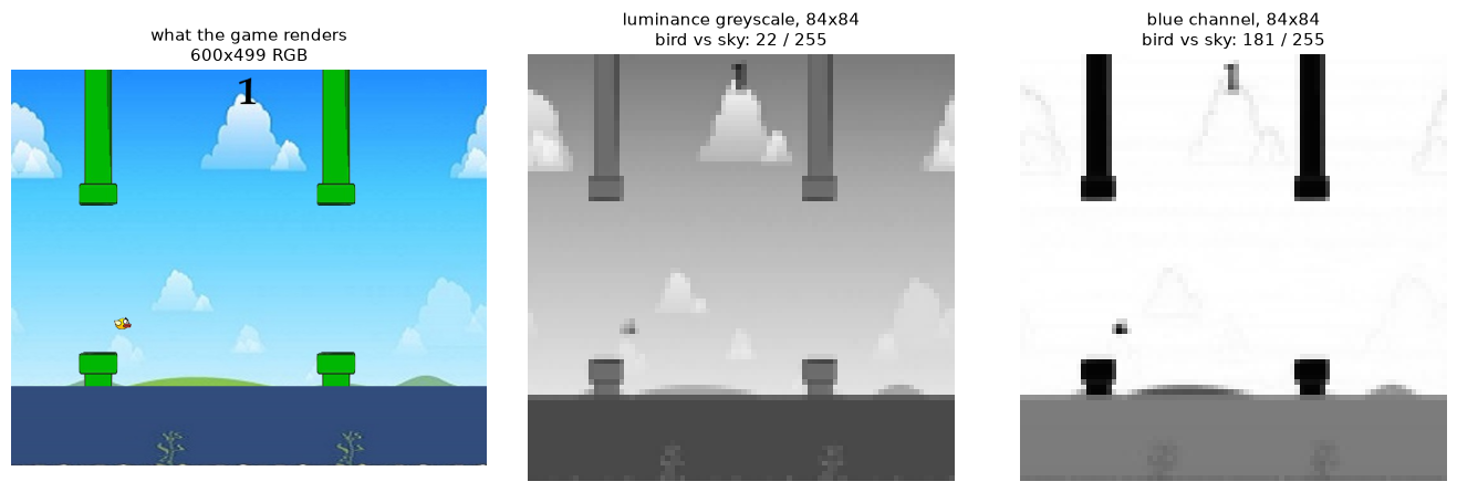
The agent plateaued for a long time and no hyperparameter fixed it. The bird is yellow, the sky is light blue, and the two are nearly equiluminant, so the standard luminance greyscale every Atari pipeline uses was giving the bird 22 levels of contrast out of 255 while the pipes got 64. Taking the blue channel instead gives 181.

The same frame as luminance greyscale and as the blue channel — Left, what the game renders. Middle, what the network was receiving. Right, what it receives now.

Learning curves for the two observation channels — Same network, same hyperparameters, same seed. Only the colour channel differs.

DQN against REINFORCE with a value baseline — REINFORCE never cleared a pipe: 756 gradient updates against the DQN's 61,250 over comparable experience.

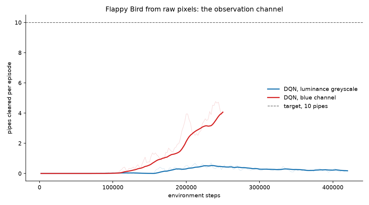
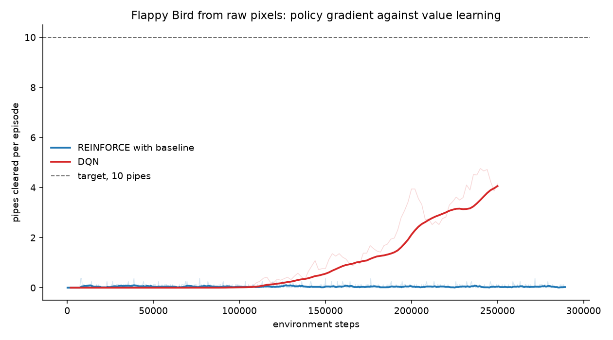
Greyscale needed 200k steps to clear its first pipe and never passed 0.80. The blue channel cleared one at 50k and passed ten at 250k. The write-up also keeps the run that failed, and a scaling bug of mine that made a value loss 224 times the policy loss.

A 3-SAT solver over GF(2)

0 wrong verdicts on 500 instances checked against exhaustive search

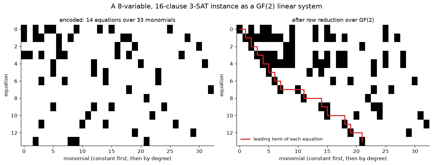
A 3-SAT instance as a GF(2) matrix, before and after row reduction — Every clause becomes a polynomial; every distinct monomial becomes an unknown. The red staircase is the leading term of each equation, which is the triangular structure the method is named for.

Clauses become polynomials over GF(2), a triangular Gröbner-style elimination propagates what it can, and branching finishes the job. Verdicts are checked by validating the returned assignment, not just the SAT or UNSAT answer.

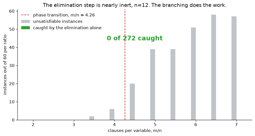
The part worth reading is where it refuses to oversell itself. The elimination step alone is sound but weak: across 285 genuinely unsatisfiable instances it flagged one, and at n=20 it resolves 0.00% of systems on its own, so essentially all the work is done by the branching. The benchmark ratio is also below the random 3-SAT phase transition, which means a high success rate there measures the instance distribution rather than the solver. The folder also keeps a paper of mine from 2023 whose central claim is wrong, with the failing line located and explained.

Unsatisfiable instances against how many the elimination caught — Across 272 unsatisfiable instances the elimination step alone caught none. Measured, not estimated.

Sorting algorithms in 3D

1407 and 801 frames at 1080p24, rendered headless in 4 and 2 minutes

Bubble sort animated in Blender — Bubble sort. The red marker walking the row again and again, one place shorter each pass, is the O(n²).

Merge sort animated in Blender — Merge sort. Recursion depth is legible as physical distance from the starting row.

Both are driven entirely from Blender's Python API and render from the command line. The scripts previously could not be rendered at all: they delete the default camera and light on their first line and set no frame range, so Blender's stock limit of 250 frames captured 18% of bubble sort against a black screen.

Matrix algorithms from scratch

11 checks against NumPy, matching to 1e-13

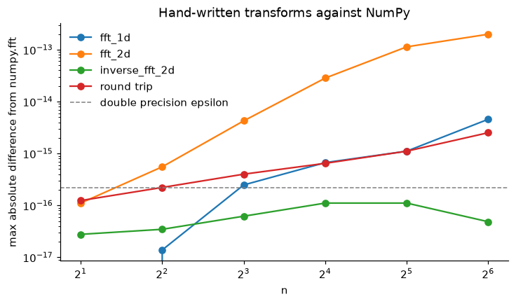
Hand-written transforms against numpy.fft — A radix-2 Cooley-Tukey transform written out, checked against `numpy.fft` up to n=64.

An FFT, a determinant through the Schur complement, an exact integer matrix inverse and a trace that never forms the product. NumPy appears throughout as the oracle each result is checked against, never as the implementation: the determinant does not call numpy.linalg.det and the transforms do not call numpy.fft.

None of them is fast, and each notebook plots its own cost so the gap is visible rather than implied. The inverse is exact rather than nearly right: A @ A_inverse is the identity, not close to it.

The French income tax, modelled

The tipping point is 59 800 EUR gross a year

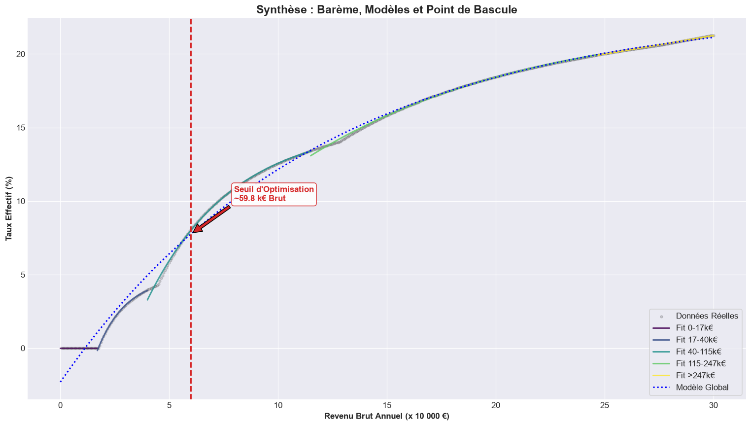
Effective tax rate against the bracket schedule, with the tipping point marked — The bracket schedule is a staircase; the rate anyone actually pays is the smooth curve underneath it.

Where does an extra euro of gross salary stop being worth much? Fitting the effective rate as an exponential approach to an asymptote and solving for where its slope stops growing needs the Lambert W function, because the equation takes the form v·e^v = c. Both branches are computed and the one that lands inside the income range is kept. Read the full report, in French.